Numpy, часть 1: начало работы
Содержание:
Operations on masked arrays
Arithmetic and comparison operations are supported by masked arrays.
As much as possible, invalid entries of a masked array are not processed,
meaning that the corresponding entries should be the same
before and after the operation.
Warning
We need to stress that this behavior may not be systematic, that masked
data may be affected by the operation in some cases and therefore users
should not rely on this data remaining unchanged.
The module comes with a specific implementation of most
ufuncs. Unary and binary functions that have a validity domain (such as
or ) return the
constant whenever the input is masked or falls outside the validity domain:
>>> ma.log()
masked_array(data=,
             mask=,
       fill_value=1e+20)
Masked arrays also support standard numpy ufuncs. The output is then a masked
array. The result of a unary ufunc is masked wherever the input is masked. The
result of a binary ufunc is masked wherever any of the input is masked. If the
ufunc also returns the optional context output (a 3-element tuple containing
the name of the ufunc, its arguments and its domain), the context is processed
and entries of the output masked array are masked wherever the corresponding
input fall outside the validity domain:
Полиномы (numpy.polynomial)
Модуль полиномов обеспечивает стандартные функции работы с полиномами разного вида. В нем реализованы полиномы
Чебышева, Лежандра, Эрмита, Лагерра. Для полиномов определены стандартные арифметические функции ‘+’, ‘-‘, ‘*’, ‘//’,
деление по модулю, деление с остатком, возведение в степень и вычисление значения полинома
Важно задавать область
определения, т.к. часто свойства полинома (например при интерполяции) сохраняются только на определенном интервале.
В зависимости от класса полинома, сохраняются коэффициенты разложения по полиномам определенного типа, что позволяет
получать разложение функций в ряд по полиномам разного типа
| Типы полиномов | Описание |
|---|---|
| Polynomial(coef) | разложение по степеням «x» |
| Chebyshev(coef) | разложение по полиномам Чебышева |
| Legendre(coef) | разложение по полиномам Лежандра |
| Hermite(coef) | разложение по полиномам Эрмита |
| HermiteE(coef) | разложение по полиномам Эрмита_Е |
| Laguerre(coef) | разложение по полиномам Лагерра |
- coef – массив коэффициентов в порядке увеличения
- domain – область определения проецируется на окно
- window – окно. Сдвигается и масштабируется до размера области определения
Некоторые функции (например интерполяция данных) возвращают объект типа полином. У этого объекта есть набор методов,
позволяющих извлекать и преобразовывать данные.
| Методы полиномов | Описание |
|---|---|
| __call__(z) | полином можно вызвать как функцию |
| convert() | конвертирует в полином другого типа, с другим окном и т.д |
| copy() | возвращает копию |
| cutdeg(deg) | обрезает полином до нужной степени |
| degree() | возвращает степень полинома |
| deriv() | вычисляет производную порядка m |
| fit(x, y, deg) | формирует полиномиальную интерполяцию степени deg для данных (x,y) по методу наименьших квадратов |
| fromroots(roots) | формирует полином по заданным корням |
| has_samecoef(p) | проверка на равенство коэффициентов. |
| has_samedomain(p) | проверка на равенство области определения |
| has_samewindow(p) | проверка на равенство окна |
| integ() | интегрирование |
| linspace() | возвращает x,y — значения на равномерной сетке по области определения |
| mapparms() | возвращает коэффициенты масштабирования |
| roots() | список корней |
| trim() | создает полином с коэффициентами большими tol |
| truncate(size) | ограничивает ряд по количеству коеффициентов |
- p – полином
- x, y – набор данных для аппроксимации
- deg – степень полинома
- domain – область определения
- rcond – относительное число обусловленности элементы матрицы интерполяции с собственными значениями меньшими данного будут отброшены.
- full – выдавать дополнительную информацию о качестве полинома
- w – веса точек
- window – окно
- roots – набор корней
- m – порядок производной (интеграла)
- k – константы интегрирования
- lbnd – нижняя граница интервала интегрирования
- n – число точек разбиения
- size – число ненулевых коэффициентов
Required subroutine
There is exactly one function that must be defined in your C-code in
order for Python to use it as an extension module. The function must
be called init{name} where {name} is the name of the module from
Python. This function must be declared so that it is visible to code
outside of the routine. Besides adding the methods and constants you
desire, this subroutine must also contain calls like
and/or depending on which C-API is needed. Forgetting
to place these commands will show itself as an ugly segmentation fault
(crash) as soon as any C-API subroutine is actually called. It is
actually possible to have multiple init{name} functions in a single
file in which case multiple modules will be defined by that file.
However, there are some tricks to get that to work correctly and it is
not covered here.
A minimal method looks like:
PyMODINIT_FUNC
init{name}(void)
{
   (void)Py_InitModule({name}, mymethods);
   import_array();
}
The mymethods must be an array (usually statically declared) of
PyMethodDef structures which contain method names, actual C-functions,
a variable indicating whether the method uses keyword arguments or
not, and docstrings. These are explained in the next section. If you
want to add constants to the module, then you store the returned value
from Py_InitModule which is a module object. The most general way to
add items to the module is to get the module dictionary using
PyModule_GetDict(module). With the module dictionary, you can add
whatever you like to the module manually. An easier way to add objects
to the module is to use one of three additional Python C-API calls
that do not require a separate extraction of the module dictionary.
These are documented in the Python documentation, but repeated here
for convenience:
- int (* module, char* name, * value)
- int (* module, char* name, long value)
7.5. Дискретное преобразование Фурье
Если данные в ваших массивах — это сигналы: звуки, изображения, радиоволны, котировки акций и т.д., то вам наверняка понадобится дискретное преобразование Фурье. В NumPy представлены методы быстрого дискретного преобразования Фурье для одномерных, двумерных и многомерных сигналов, а так же некоторые вспомогательные функции. Рассмотрим некоторые простые примеры.
Одномерное дискретное преобразование Фурье:
Двумерное дискретное преобразование Фурье:
Очень часто при спектральном анализе используются оконные функции (оконное преобразование Фурье), некоторые из которых так же представлены в NumPy
7.1. Базовые математические операции
Пожалуй, первое с чего стоит начать, так это с того, что массивы NumPy могут быть обычными операндами в математических выражениях:
Для выполнения таких операций на Python, мы были вынуждены писать циклы. Писать такие циклы в NumPy, нет никакой необходимости, потому что все операции и так выполняются поэлементно:
Точно так же обстоят дела и с математическими функциями:
Такие операции как , , , и прочие подобные, могут применяться к массивам и так же выполняются поэлементно. Они не создают новый массив, а изменяют старый:
При работе с массивами разного типа, тип результирующего массива приводится к более общему:
Применение логических операций к массивам, так же возможно и так же выполняется поэлементно. Результатом таких операций является массив булевых значений ( и ):
Мы уже знаем что массив и число могут быть операндами самых разных математических выражений:
Операндами могут быть даже несколько различных массивов, правда их размеры должны быть одинаковыми:
Хотя, если честно, их размеры должны быть не равны, а должны быть совместимыми. Если их размеры совместимы, т.е. один массив может быть растянут до размеров другого, то в дело включается механизм транслирования массивов NumPy. Этот механизм очень прост, но имеет весьма специфичные нюансы. Рассмотрим простой пример:
В данном примере массив b может быть растянут до размеров массива a и станет абсолютно идентичен массиву c. Транслирование массивов невероятно удобно, так как позволяет избежать создания множества вложенных и невложенных циклов. К тому же в NumPy этот механизм реализован для максимально быстрого выполнения. Так что используйте транслирование везде, где это возможно в ваших вычислениях.
Вычисление суммы всех элементов в массиве и прочие унарные операции в NumPy реализованы как методы класса :
По умолчанию, эти операции применяются к массиву как к обычному списку чисел, без учета его ранга (размерности). Но если указать в качестве параметра одну из осей , то вычисления будут производиться именно по ней:
Extended Precision
Python’s floating-point numbers are usually 64-bit floating-point numbers,
nearly equivalent to . In some unusual situations it may be
useful to use floating-point numbers with more precision. Whether this
is possible in numpy depends on the hardware and on the development
environment: specifically, x86 machines provide hardware floating-point
with 80-bit precision, and while most C compilers provide this as their
type, MSVC (standard for Windows builds) makes
identical to (64 bits). NumPy makes the
compiler’s available as (and
for the complex numbers). You can find out what your
numpy provides with .
NumPy does not provide a dtype with more precision than C’s
; in particular, the 128-bit IEEE quad precision
data type (FORTRAN’s ) is not available.
For efficient memory alignment, is usually stored
padded with zero bits, either to 96 or 128 bits. Which is more efficient
depends on hardware and development environment; typically on 32-bit
systems they are padded to 96 bits, while on 64-bit systems they are
typically padded to 128 bits. is padded to the system
default; and are provided for users who
want specific padding. In spite of the names, and
provide only as much precision as ,
that is, 80 bits on most x86 machines and 64 bits in standard
Windows builds.
Be warned that even if offers more precision than
python , it is easy to lose that extra precision, since
python often forces values to pass through . For example,
the formatting operator requires its arguments to be converted
to standard python types, and it is therefore impossible to preserve
extended precision even if many decimal places are requested. It can
be useful to test your code with the value
.
Recommendations
We’ll start with recommendations based on the user’s experience level and
operating system of interest. If you’re in between “beginning” and “advanced”,
please go with “beginning” if you want to keep things simple, and with
“advanced” if you want to work according to best practices that go a longer way
in the future.
Beginning users
On all of Windows, macOS, and Linux:
- Install Anaconda (it installs all
packages you need and all other tools mentioned below). - For writing and executing code, use notebooks in
JupyterLab for
exploratory and interactive computing, and
Spyder or Visual Studio Code
for writing scripts and packages. - Use Anaconda Navigator to
manage your packages and start JupyterLab, Spyder, or Visual Studio Code.
Windows or macOS
- Install Miniconda.
-
Keep the conda environment minimal, and use one or more
to install the package you need for the task or project you’re working on.
- Unless you’re fine with only the packages in the channel, make
your default channel via .
Linux
If you’re fine with slightly outdated packages and prefer stability over being
able to use the latest versions of libraries:
- Use your OS package manager for as much as possible (Python itself, NumPy, and
other libraries). - Install packages not provided by your package manager with .
If you use a GPU:
- Install Miniconda.
-
Keep the conda environment minimal, and use one or more
to install the package you need for the task or project you’re working on.
- Use the conda channel ( doesn’t have good support for
GPU packages yet).
Otherwise:
- Install Miniforge.
-
Keep the conda environment minimal, and use one or more
to install the package you need for the task or project you’re working on.
Alternative if you prefer pip/PyPI
For users who know, from personal preference or reading about the main
differences between conda and pip below, they prefer a pip/PyPI-based solution,
we recommend:
- Install Python from, for example, python.org,
Homebrew, or your Linux package manager. - Use Poetry as the most well-maintained tool
that provides a dependency resolver and environment management capabilities
in a similar fashion as conda does.
Operations on masked arrays
Arithmetic and comparison operations are supported by masked arrays.
As much as possible, invalid entries of a masked array are not processed,
meaning that the corresponding entries should be the same
before and after the operation.
Warning
We need to stress that this behavior may not be systematic, that masked
data may be affected by the operation in some cases and therefore users
should not rely on this data remaining unchanged.
The module comes with a specific implementation of most
ufuncs. Unary and binary functions that have a validity domain (such as
or ) return the
constant whenever the input is masked or falls outside the validity domain:
>>> ma.log()
masked_array(data=,
             mask=,
       fill_value=1e+20)
Masked arrays also support standard numpy ufuncs. The output is then a masked
array. The result of a unary ufunc is masked wherever the input is masked. The
result of a binary ufunc is masked wherever any of the input is masked. If the
ufunc also returns the optional context output (a 3-element tuple containing
the name of the ufunc, its arguments and its domain), the context is processed
and entries of the output masked array are masked wherever the corresponding
input fall outside the validity domain:
Examples: how to use numpy arange
Now, let’s work through some examples of how to use the NumPy arange function.
Before you start working through these examples though, make sure that you’ve imported NumPy into your environment:
# IMPORT NUMPY
import numpy as np
Ok, let’s get started.
Create a simple NumPy arange sequence
First, let’s use a simple case.
Here, we’re going to create a simple NumPy array with 5 values.
np.arange(stop = 5)
Which produces something like the following array:
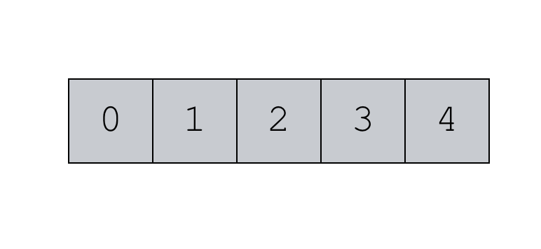
Notice a few things.
First, we didn’t specify a value. Because of this, the sequence starts at “0.”
Second, when we used the code , the “5” serves as the position. This causes NumPy to create a sequence of values starting from 0 (the value) up to but excluding this stop value.
Next, notice the spacing between values. The values are increasing in “steps” of 1. This is because we did not specify a value for the parameter. If we don’t specify a value for the parameter, it defaults to 1.
Finally, the data type is integer. We didn’t specify a data type with the parameter, so Python has inferred the data type from the other arguments to the function.
One last note about this example. In this example, we’ve explicitly used parameter. It’s possible to remove the parameter itself, and just leave the argument, like this:
np.arange(5)
Here, the value “5” is treated a positional argument to the parameter. Python “knows” that the value “5” serves as the point of the range. Having said that, I think it’s much clearer to explicitly use the parameter names. It’s clearer if you just type .
Create a sequence in increments of 2
Now that you’ve seen a basic example, let’s look at something a little more complicated.
Here, we’re going to create a range of values from 0 to 8, in increments of 2.
To do this, we will use the position of 0 and a position of 2. To increment in steps of 2, we’ll set the parameter to 2.
np.arange(start = 0, stop = 8, step = 2)
The code creates a object like this:
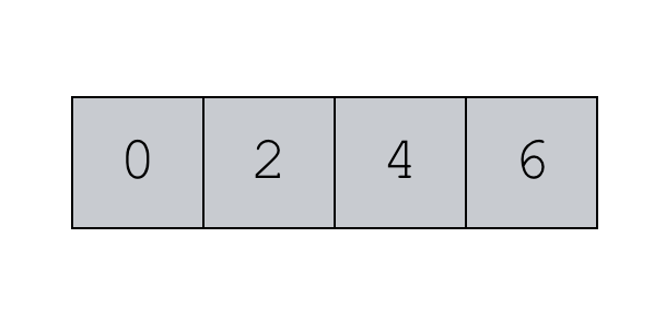
Essentially, the code creates the following sequence of values stored as a NumPy array: .
Let’s take a step back and analyze how this worked. The output range begins at 0. This is because we set .
The output range then consists of values starting from 0 and incrementing in steps of 2: .
The range stops at 6. Why? We set the parameter to 8. Remember though, numpy.arange() will create a sequence up to but excluding the value. So once arange() gets to 6, the function can’t go any further. If it attempts to increment by the step value of 2, it will produce the value of 8, which should be excluded, according to the syntax . Again, np.arange will produce values up to but excluding the value.
Specify the data type for np.arange
As noted above, you can also specify the data type of the output array by using the parameter.
Here’s an example:
np.arange(start = 1, stop = 5, dtype = 'float')
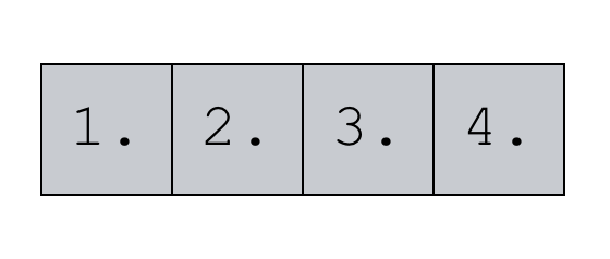
First of all, notice the decimal point at the end of each number. This essentially indicates that these are floats instead of integers.
How did we create this? This is very straightforward, if you’ve understood the prior examples.
We’ve called the np.arange function starting from 1 and stopping at 5. And we’ve set the datatype to float by using the syntax .
Keep in mind that we used floats here, but we could have one of several different data types. Python and NumPy have a couple dozen different data types. These are all available when manipulating the parameter.
Create a 2-dimensional array with np.arange
It’s also possible to create a 2-dimensional NumPy array with numpy.arange(), but you need to use it in conjunction with the NumPy reshape method.
Ultimately, we’re going to create a 3 by 3 array with the values from 1 to 9.
But before we do that, there’s an “intermediate” step that you need to understand.
…. let’s just create a 1-dimensional array with the values from 1 to 9:
np.arange(start = 1, stop = 10, step = 1)
This code creates a NumPy array like this:

Notice how the code worked. The sequence of values starts at 1, which is the value. The final value is 9. That’s because we set the parameter equal to 10; the range of values will be up to but excluding the value. Because we’re incrementing in steps of 1, the last value in the range will be 9.
Ok. Let’s take this a step further to turn this into a 3 by 3 array.
Here, we’re going to use the reshape method to re-shape this 1-dimensional array into a 2-dimensional array.
np.arange(start = 1, stop = 10, step = 1).reshape((3,3))
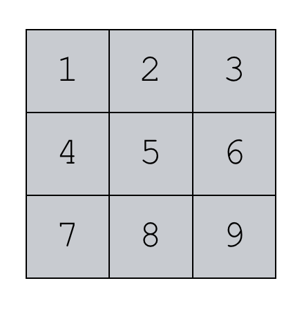
Notice that this is just a modification of the code we used a moment ago. We’re using to create a sequence of numbers from 1 to 9.
Then we’re calling the method to re-shape the sequence of numbers. We’re reshaping it from a 1-dimensional NumPy array, to a 2-dimensional array with 3 values along the rows and 3 values along the columns.